Notebooks
Within the notebooks/ directory, you will find as series of [Jupyter Notebooks](https://www.jupyter.org) that demonstrate how to use playNano programmatically in an interactive environment. These notebooks cover the entire workflow from loading and processing data to analysis and export.
These are useful as it allows the user to explore interactively and with rapid feedback the parameters that may need adjusting in order to process a high-speed dataset. The notebooks can be found in the notebook/ directory after cloning the GitHub repository.
To access these notebooks you will need to clone the playNano repository from [GitHub](https://github.com/derollins/playNano)
and install the optional notebook dependencies using pip install .[notebooks].
git clone https://github.com/derollins/playNano.git   # Clone the repository
cd playNano
pip install -e . [notebooks]  # Install the package and notebook dependencies
Current notebooks:
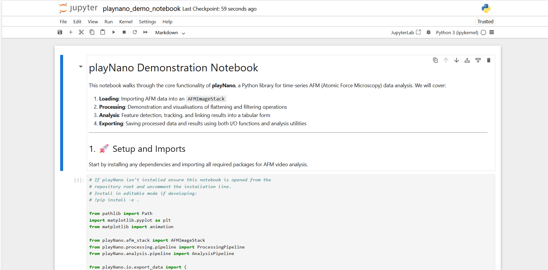
playnano_demo_notebook.ipynb: An overview of loading, processing, analysing, and exporting time-series AFM data using the playNano library API.
processing_demo.ipynb: A step-by-step guide to applying processing filters and exploring and exporting results.
Running Notebooks
Once installed Jupyter can be launched from the command line.
jupyter notebook
This will open a browser window where you can navigate to the notebooks/ directory and open the notebooks.
Run each cell in the notebooks sequentially to see the workflow in action. Initially example data from the test folder is used however you can change the paths to examine your own data and modify the processing and analysis steps to begin to analyse your data.
The full API reference is available in the API Reference section of the documentation.